![]()
![]()
All files distributed with LGL fall under the terms of the GNU General Public License, and are copyright (c) 2002, 2003 Alex Adai.
Changes and updates copyright (c) 2004-2022 Barrett Lyon
LGL on the web at: http://www.opte.org/
If you use this in your research, please cite (if possible):
- Lyon, Barrett. "The Opte Project." Mapping the Internet, Self, 2003-2022. http://www.opte.org.
- Adai, Alex T., Shailesh V. Date, Shannon Wieland, and Edward M. Marcotte. “LGL: Creating a Map of Protein Function with an Algorithm for Visualizing Very Large Biological Networks.” Journal of Molecular Biology 340, no. 1 (2004): 179–90. https://doi.org/10.1016/j.jmb.2004.04.047.
Note: Most of the Perl contained in this package is no longer maintained. The Java and C++ components are "mostly" modernized.
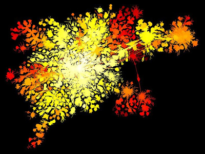
Protein Homology Graph, Edward Marcotte and Alex Adai, MoMA

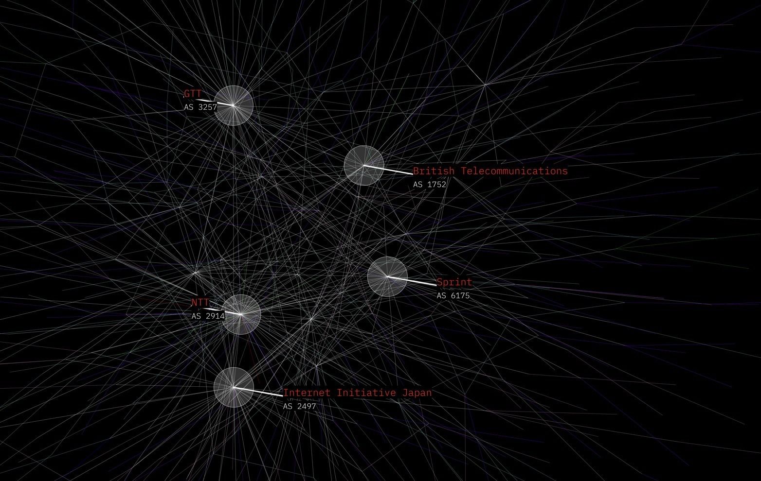
Internet using traceroute vs BGP in 2003, Barrett Lyon, MoMA
A heap of stuff, in no particular order:
- A C++ compiler
- Boost library required (I should have fixed version issues, but I have not future proofed it)
- bgpdump (https://bitbucket.org/ripencc/bgpdump/wiki/Home)
- Also see bgpscanner (Works with threads and is faster than bgpdump)
- perl (5+, I think)
- Java (openjdk version "11.0.16" 2022-07-19)
- Xserver installed for graphical tools (works well under WSL 2 in Windows)
- Graphical tools also work on anything with Java.
- Python 3 (there are bash scripts lying around as well, but the python scripts are 3x faster)
- Only used for example scripts
- User guide to LGL:
- Getting up to speed on Internet routing:
prompt$ setup.pl -i

This script which does a lot of suspect lifting.
This will compile 2D and 3D versions of LGL and put the resulting binaries in the ./bin directory. Afterwards you can move them whereever you want.
NOTE: setup.pl has been updated to locate boost, however you may need to direct gcc on where to find the includes if the automated detection does not work:
env CPLUS_INCLUDE_PATH=/usr/local/include ./setup.pl -i
Use the gmake Makefile, i.e.
prompt$ make
prompt$ make install # local install in $(PROJECTDIR)/bin
(If you intend to use these scrips)
You must have the following Perl modules in your @INC path to run LGL:
ParseConfigFile.pm
LGLFormatHandler.pm
These files are in the ./perls directory. You don't have to know anything about these modules, and you won't have to use them directly but lgl.pl will call them.
After all is compiled and done you can run LGL by the driver script lgl.pl as:
prompt$ ./bin/lgl.pl edges_file
but you have to modify the 'tmpdir' variable in lgl.pl. That directory will
hold all the files that LGL outputs, and it must be changed for EACH run.
However, The best way to run LGL is to have setup.pl generate a sample
config file for lgl.pl by running it as
prompt$ ./setup.pl -c conf_file_name
That file (after modification of course) can just be given to lgl.pl for execution as follows:
prompt$ ./bin/lgl.pl -c conf_file_name
The config file itself is documented further, and explains each of the variables to be used. It also provides defaults, so the minimum that MUST be changed are the variables:
tmpdir
inputfile
where tmpdir is the output directory of the LGL run and inputfile is the edge file. inputfile must be a file parsable by LGLFormatHandler.pm This can be just a simple 2 column space delimited file with one edge per line (the 2 vertex ids represent the two columns).
One last change is to ./bin/lgl.pl. A Perl variable $LGLDIR must be set to the root bin directory of all the lgl executables (This might be /where/lgl/was/unpacked/bin ). This var is empty by default, and the program won't run until it is set correctly.
A list of important files in the perls dir:
genVrml.pl - This generates the VRML code from 3D layout results. Run
genVrml.pl with no args to get the usage.
colorEdgesBasedOnLevel.pl - This generates a simple color file to be given to lglview, that will color your edges based on the level in the heirarchy in layout.
Other files might be included as well, but they are not necessary for LGL. Their documentation will be added here in the near future, or they may not be carried in the future.
This is the core of LGL and generates the coords file for image generation.
Usage: ./lgl-exparmental-label/bin/lglayout2D [-x InitPositionFile] [-a AnchorsFile] [-t ThreadCount] [-m InitMassFile] [-i IterationMax] [-s] [-r nbhdRadius] [-T timeStep] [-S nodeSizeRadius] [-k casualSpringConstant] [-s specialSpringConstant] [-e] [-l] [-y] [-q EQ Distance] [-u placementDistance] [-E ellipseFactors] [-v placementRadius] [-L] nodeFile.lgl
    -[mx]    A file that has the node id followed by
            the initial values.

        -t      The number of threads to spawn.
                This is capped by the processor count.

        -i      The maximum number of iterations.

        -r      The neighborhood radius for each particle. It
                defines the interaction range for casual (generally
                repulsive) interactions

        -T      The time step for each iteration

        -S      The 'radius' of each node.

        -M      The 'mass' of each node.

        -R      The radius of the outer perim.

        -W      The write interval.

        -z      Root node you want to use.

        -l      Write out the edge level map.

        -e      Output the mst used.

        -O      Use original weights.

        -y      Layout the tree only.

        -I      Don't show layout progress, be quiet (kinda)

        -q      Equilibrium distance.

        -E      Ellipse factors. (Force the layout to be more of an ellipse -E 1x1.2)

        -u      Placement distance is the distance you want
                the next level to be placed with respect to
                the previous level. If this float value is not
                given a formula calculates the placement distance.

        -v      Placement radius is a measure of the placement density

        -L      Place the leafs close by. This applies to trees more than
                graphs. Setting this option will place the child vertices very
                near the parent vertex if all of its children have none themselves.

        -o      Read a previously created coordinates file to start processing level processing. This technique is used for animations.
Generating Static Images using LGLLib.jar
Runtime Example:
java -Djava.awt.headless=true -Xmx20000m -Xms20000m -cp ./LGL-Master/Java/jar/LGLLib.jar ImageMaker.GenerateImages <height> <width> run.lgl run.coords -c run.colors -s 0.01 -l run.labels

-c <colors file>
-s Scale for labels
-l <labels file>
-M x,y (max of x and y to control scale and zoom. Not required)
-m x,y (min of x and y to control scale and zoom. Not required)
-a center (not required, align the mean of the image to the center of the window)
To use the -M and -m features you can get the min and max values from rendering the largest graph in your series. You can use the largest graph's min/max values on the smallest series to keep perspective rather than a fit-to-screen zoom.
Looking at the huge PNG (100k x 100k pixels) java.awt.image.Raster: The maximum width x height has to be less than Integer.MAX_VALUE (2147483647) so the maximum square image is 46340 x 46340. Note also that such images will need a lot of RAM since Java's BufferedImage's pixels are hold in memory.
An example of a larger output would be:
java -Djava.awt.headless=true -Xmx5G -Xms5G -cp ./LGL-Master/Java/jar/LGLLib.jar ImageMaker.GenerateImages 29200 29200 <files...>
coordinates use LGLLib.jar
java -Xmx2G -Xms2G -cp ./LGL-master/Java/jar/LGLLib.jar Viewer2D.Viewer2D
Shortcuts

(Thank you to Claire McWhite for major parts of this tutorial)
The input format to LGL is called .ncol, which is just a space separated list of two connected nodes with an optional third column of weight.
$ cat example.lgl
node1 node2 [optional weight]
Key points for formatting the input .ncol

Each line must be unique
A node may connect to many other nodes
A node cannot connect to itself
If a line is B-A, there cannot also be a line A-B
There can’t be blank lines
There can’t be blanks in any column
No header line
node1 node2
node1 node3 # OK
node1 node2 # Will cause error
node1 node1 # Will cause error
node2 node1 # Will cause error
node3         # Will cause error
          # Trailing blank line will cause error
LGL allows you to color both nodes and edges. In order to color edges, each pairwise edge must have an R G B value. To color individual nodes, each node must have an R G B value. RGB values must be scaled to one 1, so just divide each number of an RGB value by 255. The rules for formatting an .ncol file apply here too, i.e. no blanks, no empty lines, no redundancy, etc.
LGL also now supports colors in hex values and is backward compatible with the previous RGB format.
$ cat example.edge.colors
node1 node2 1.0 0.5 0.0
node3 node4 0.0 1.0 0.8
node5 node6 0.1 0.1 1.0

or

$ cat example2.edge.colors
node1 node2 FFFFFF FFFFFF FFFFFF
node3 node4 0.0 1.0 0.8
node5 node6 0.1 0.1 1.0


$ cat example.vertex.colors
node1 1.0 0.8 0.0
node2 1.0 0.5 0.0
node3 0.2 0.1 0.8
node4 0.0 1.0 0.8
node5 0.6 0.5 0.5
node6 0.1 0.1 1.0
LGL now supports labels! It's a flat file with single line entries for the configuration of each label with a \n at the end.
Pixel sizes cannot be in decimal or fractions
Colors will be referenced by their hex values. 000000-111111 (Do not include the #)
NULL values will delete the segment of the label: shape, line, text1, text2
Example of image generated with labels.
nodename,
	(name of the node we want to center the shape around)
shape,
	(name of shape: circle or square)
shape_size,
	(size of the shape in pixels from center to edge?)
shape_border_with,
	(width of the shape in px)
shape_border_color,
	(color used for the shape border)
shape_fill_color,
	(color used to fill the shape)
shape_fill_opacity,
	(opacity for the fill of the shape)
line_size,
	(width of line in px)
line_length,
	(length of line in px)
line_angle,
	(direction of the line off the shape edge)
line_color,
	(color of the line off the shape)
top_text_ttf,
	(full path filename for ttf font)
top_text_size,
 	(text size)
top_text_color,
 	(text color for upper text)
top_bg_fill_color
	(color used for text background)
bottom_text_ttf,
	(full path filename for ttf font)
bottom_text_size,
 	(text size)
bottom_text_color,
	(text color for upper text)
bottom_bg_fill_color
	(color used for text background)
top_text
	(text string for top label)
Bottom_text
	(text string for bottom label)
Example of a label in the input config file:
174,circle,20,2,000000,000000,100,5,25,30,000000,file.ttf,25,FFFFFF,000000,file.ttf,50,FFFFFF,000000,COGENT COMMUNICATIONS,GLOBAL NETWORK
Command line example:
java -Djava.awt.headless=true -Xmx20000m -Xms20000m -cp ./LGL-master/Java/jar/LGLLib.jar ImageMaker.GenerateImages 5000 5000 <file.lgl> <file.coords> -c <file.colors> -l <file.labels> -s <scale ex: 0.1>
For Opte we parse the output of BGP into an .ncol (.lgl) file format, a .color file, and a .label file. The lgl file is read into lglayout2D, which creates the .coords output file. These combined are read by the ImageMaker Java application to output an image.
To create an animation, each step in the data set is incremental in time. Thus to generate the next frame in the animation, the -o option is used to read in the previous .coords file. The last file is used to set up the landscape and processes the changes from one dataset to the next.
Once all the images are complete, they can be combined as an animation using FFMpeg.
Data parsing -> lglayout2d -> ImakeMaker -> Animation
This is any example to make a network with colored nodes and edges. I would begin by making a file of all pairwise edges and their associated traits. It can be difficult to keep .ncol and .color files in sync, and so it will cause fewest headaches to begin with one file containing all the information to create both.
$ echo "Nodes and traits"
$ cat homology.txt
node1 node2 source score rank species1 species2
protein1 protein2 blastp 150 1 mouse human
protein3 protein4 blastp 50 2 wheat rat
protein2 protein5 hmmscan 60 3 human human
Then take the first two columns (minus the header) to create an .ncol file. This is the file used to layout the graph

$ echo "Get node columns, remove header"
$ awk '{print $1, $2}' homology.txt  | awk '{if(NR>1)print}' > homology.ncol
$ cat homology.ncol
protein1 protein2
protein3 protein4
protein2 protein5
Then choose a trait, and create a edge.colors file. I generally select the first two columns, and a trait to color by, then just use sed to replace the trait values with the RGB value I want to color that type of edge by.
In this file, we want to color all edges predicted with the algorithm hmmscan red, and all edges found with blastp blue.
$ echo "Get node columns and trait column"
$ awk '{print $1, $2, $3}' homology.txt  | awk '{if(NR>1)print}' >  homology_alg.colors.tmp

$ echo "Replace hmmscan trait with RGB value
$ sed -i 's/hmmscan/0 1 0/g' homology_alg.colors.tmp

$ echo "Replace blastp trait with RGB value
$ sed 's/blastp/0 0 0/g' homology_alg.colors.tmp > homology_algorithm.edge.colors

$ cat homology_algorithm.edge.colors
protein1 protein2 0 0 0
protein3 protein4 0 0 0
protein2 protein5 0 1 0
We could also color each node by some trait. In this file format, each vertex must have an associated RGB value. In this case, we want to color every human protein red, and proteins from every other species blue.
$ echo "Get first column of nodes and species"
$ awk '{print $1, $6}' homology.txt  | awk '{if(NR>1)print}'> vertex1_species.tmp

$ Get second column of nodes and species"
$ awk '{print $2, $7}' homology.txt  | awk '{if(NR>1)print}'> vertex2_species.tmp

$ Get unique nodes"
$ cat vertex1_species.tmp vertex2_species.tmp | sort -u > homology_human.vertex.colors.tmp

$ Color human nodes red"
$ sed -i 's/human/1 0 0/' homology_human.vertex.colors.tmp

$ Color any other node blue"
$ sed 's/mouse\|wheat\|rat/0 0 1/' homology_human.vertex.colors.tmp > homology_human.vertex.colors

$ cat homology.human.vertex.colors
protein1 0 0 1
protein3 0 0 1
protein2 1 0 0
protein4 0 0 1
protein5 1 0 0
Running
The Opte Project was able to use lglayout2D to create a full animation in 10k using this new pre-seeding technique:
./LGL-master/bin/lglayout2D -D -t 56 -x <filename for the previous frame coords file> -o <run.coords> -E1x1.2 run.lgl
LGL will read the previous file and start with those coordinates rather than starting from scratch. This technique allows nodes to stay in nearly the same place creating another frame generated from the previous.
The most obvious way to expand LGL is to add support for your type of edge file to LGLFormatHandler.pm. Just add a method to read in your file type, update the 'loadFromFile' method to recognize your file suffix, and that should be it.
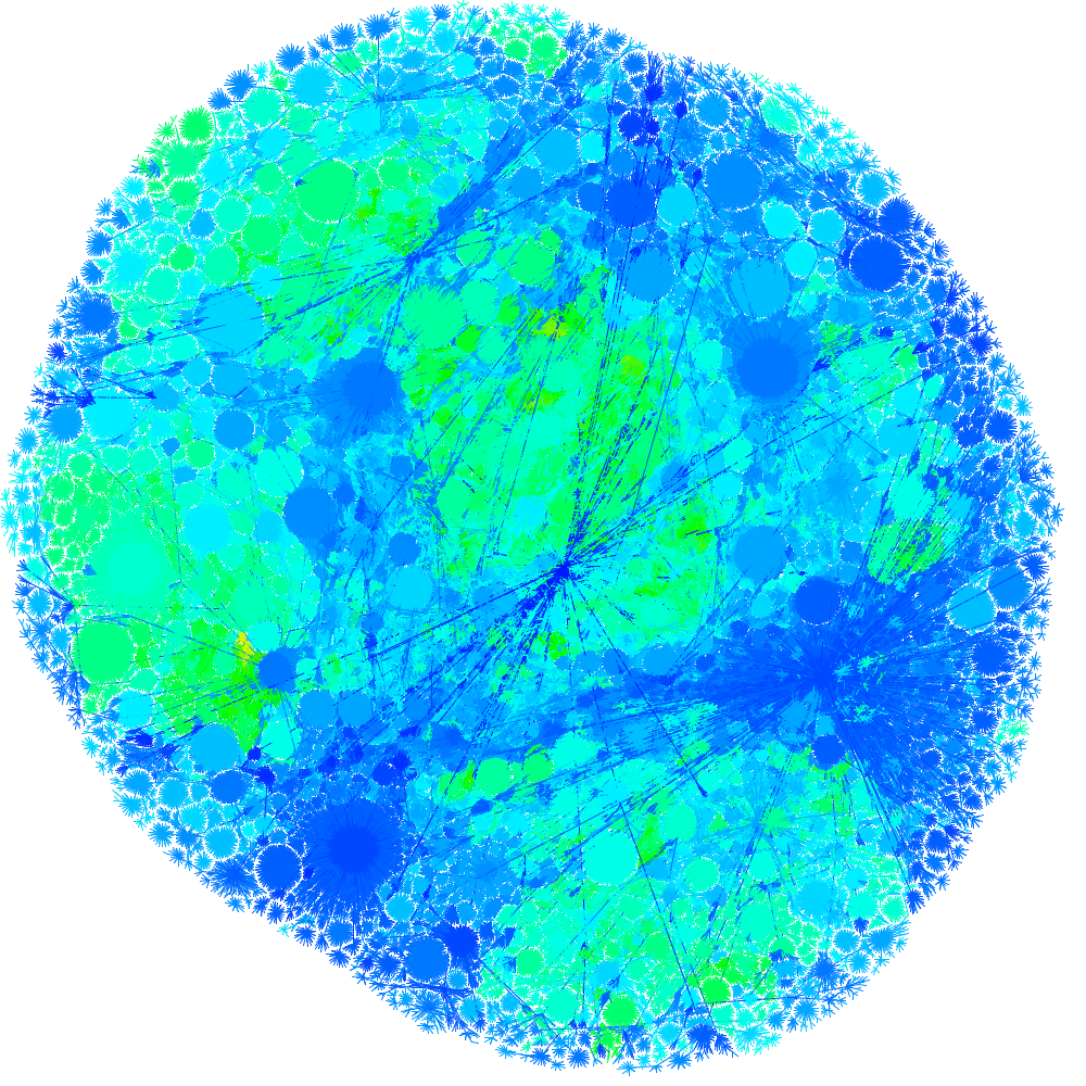
An example of the Internet as generated by data from 2016. Lindeberg, Fredrik
These scrips and changes are copyright (c) 2019, 2020 Fredrik Lindeberg
If your intention is to graph custom stuff, just hack away. Below is how you quite easily can make graphs from bgp-dumps. You need a separate folder for each project, due to design in the original LGL library. Below follows an example for a graph for a 2000 Internet. Takes around 10 minutes on a fairly modern computer (8 threads or so) with a decent Internet connection.
The oneliner which creates a graph, including bootstrapping, from 2000-09-01:
prompt$ cd scripts/
prompt$ ./creategraphfromdate.sh 2000 09
prompt$ # doing magic, and creating a graph
prompt$ # arguments to creategraphfromdate are year and month
prompt$ # and the scipt lacks proper error handling
The same thing but step by step (if above fails):
prompt$ cd scripts/
prompt$ ./create_run.sh internet_2000
prompt$ cd ../testrun/internet_2000
prompt$ wget http://data.ris.ripe.net/rrc00/2000.09/bview.20000901.0610.gz
prompt$ ./bootstrap.sh bview.20000901.0610.gz
prompt$ # doing magic, and creating a graph
prompt$ # by default generating a 2400x2400 png (change run.sh for different resolution)
prompt$ # should be a 'internet_2001.png' in 'testrun/internet_2001' if all went well
Also possible:
prompt$ cd scripts/
prompt$ ./creategraphfromurl.sh http://data.ris.ripe.net/rrc00/2000.09/bview.20000901.0610.gz
prompt$ # wait for magic, by default generating a 2400x2400 png (change run.sh for different resolution)
prompt$ # should be a 'view.20000901.0610.png' in 'testrun/bview.20000901.0610' if all went well
Replace the bview-file with a more recent one for a larger and newer network network. Coloring is
set in perls/colorEdgesBasedOnLevel.pl, currently a mix of greenish and bluish tints going on white
at the edges.
A short disclaimer; the graph is only as good as your data. The bootstrap script works for generating interesting graphs. Are they 100% correct? I don't know, you are welcome to check and improve the code! There might be BGP-quirks I do not know of, even though I catch the vast majority of bgp announcements.